Having recently read about recurrent neural networks (RNNs) and an excellent blog post about using recurrent neural networks to emulate Shakespeare’s writing, I thought it would be a kind of cool to see if a recurrent neural network can be trained to create Bollywood songs. For those unfamiliar with Bollywood, it refers to the Hindi movie industry based in Mumbai, formerly known as Bombay, in India. Bollywood churns out around 1,000 movies per year, thus making it the biggest center of movie production in the world. Bollywood movies are known for songs and dances. While the present day Bollywood movies tend to have only two or three songs, there was a time when eight to ten songs in a movie was routine. Thus there are hundreds of thousands of Hindi movie songs and most of them can be found on Youtube. Since interest in these songs is high not only in India but across the globe, there are websites where one can find the lyrics of these movie songs in Hindi as well as in Roman Hindi, Hindi written using Roman alphabet, and also in many other languages. Figure 1 gives an example of lyrics of a Bollywood movie song written both in Devanagari script and in Roman script. Thus, creating a corpus of Hindi songs is not a difficult task. So this blog post is about training a recurrent neural network with Bollywood songs inputted in Roman Hindi and the results obtained. Before I get into details, let me provide a brief introduction to recurrent neural networks.

What is a Recurrent Neural Network?
When we think of feedforward neural networks, we typically do not associate any memory capabilities with such networks; this is because the output of such networks at any given instant is 100% dependent upon input at that instant and the connection weights. However, there are numerous situations where we want the network to remember its recent history of inputs and respond accordingly. Such networks are known as recurrent neural networks. To see how information about previous inputs to a neural network can be retained, let us consider the feedforward neural network consisting of three input and two hidden layer neurons as shown in Figure 2.

Let WI be the weight matrix which represents the connection weights between the three input neurons and the two hidden neurons H1 and H2. Suppose the weight matrix is given by the following values.
WI =
-0.197705 -0.703846
-0.232759 -0.084652
0.462215 -0.858601
Assume the input neurons are fed the values as shown at time instant t. With sigmoidal activation function for hidden neurons, H1 and H2 will produce the following output at time instant t. (Bias term is ignored in all calculations)
H1 = 0.57855; H2 = 0.22663
Let WO = [0.30716 0.50222]T represent the connection weights between the hidden layer neurons and the output later. Then the output neuron with sigmoidal activation yields 0.74712 as the network output at time instant t.
Now let us make a change in the configuration of the network of Figure 2 to obtain the network of Figure 3. The change consists of taking the outputs of the hidden neurons and feeding them back via after a unit time delay. Let the weights of the hidden layer to hidden layer feedback links be given by matrix WH. In this case it is a 2×2 matrix. Let this matrix be
WH =
-0.677205 -0.588996
-0.969968 -0.060021

Now suppose we apply the same input at next time instant, that is at time t+1. In this case, the hidden neurons will produce the following output: H1 = 0.44807; H2 = 0.14158; and the network output at time t+1 will be 0.81161, different from the output at time t although it is the same input at times t and t+1. This is due to the feedback connections in the hidden layer with unit time delay. These feedback connections are called recurrent connections and the architecture of Figure 3 represents simple recurrent neural networks.
It can be easily visualized that as newer inputs at times t+2, t+3, and so on are applied, the contribution of the input at time instant t persists in the network but it fades away slowly. This persistence of the input at time t over few following inputs is what gives rise to memory capability of the network. Often, the persistence of input at time t over successive time-steps is shown by drawing an unrolled representation of recurrent neural networks as shown in Figure 4. In this figure, each neural network block is similar to the feedforward network of Figure 2 and the recurrent connections of Figure 3 (shown as dotted lines) are represented by left to right arrows connecting neural network blocks. We can train such networks using the backpropagation algorithm once the training data specifies the input sequence and the corresponding output sequence.

To illustrate the use of a recurrent neural network, let us consider predicting the gray level of next pixel given the current pixel along a row in an image. Remember that gray levels have a strong correlation with successive pixel values except at discontinuities (where edges are present in an image). Thus, this prediction problem is a good candidate for using a recurrent neural network. A plot of normalized gray level values along a row taken from an image is shown in Figure 5.
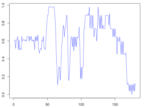
I used this as input to the rnn package in R to predict the next pixel value. The results from a run where the number of hidden neurons was set to 12 and 1200 epochs is shown in Figure 6. It is seen that the network is able to predict reasonably well except at those pixels where the gray level jumps suddenly due to an edge in the image.

Long Short-Term Memory (LSTM) Networks
An issue with simple RNN architecture is that it has difficulties memorising long term associations. For example, if you are interested in using RNNs for language modeling to predict next word in a sentence, its not good enough to just look at the current word. Better results are obtained by keeping track of few earlier words to build long term associations. The main source of this deficiency of RNNs not being able to learn long term associations is the vanishing gradient problem wherein the gradient magnitude either becomes too large or too small during the first or last time steps in training. To tackle the vanishing gradient problem and make the network suitable for remembering history over longer duration, LSTM model was introduced by Hochreiter and Schmidhuber in 1997. Since then, some changes have been incorporated in the model.
The original LSTM model replaced each hidden layer neuron of RNN architecture with a memory cell consisting of three sigmoidal neurons, two product or multiplier units, and a linear unit with a recurrent connection of fixed unit weight. The recurrent connection with a fixed weight in each cell ensures that gradient values over successive time steps can move freely without being amplified or decimated. Later on, an additional sigmoidal unit was added to the cell. It was also found that using the hyperbolic tangent nonlinearity in place of the sigmoidal nonlinearity in one of the neurons led to better results. A memory cell of LSTM network as used at present is shown in Figure 7.

Looking at the diagram of a LTSM cell, we see lines/links of two distinct colors to represent signals at current time step t and previous time step t-1. The neuron unit with tanh activation function, gct, is called the input node; it functions just like a hidden neuron unit in an RNN by taking the current input xt from input layer and the output of the hidden layer cells, ht-1, from previous time step. The neuron unit on immediate right to the input node is termed input gate. It also receives current input and previous time step output from hidden layer. The output of this unit is used to control the input reaching the linear unit with recurrent connection, sct, shown in the center of the cell diagram. This is done by running the outputs of the input node and input gate units through a multiplier shown with symbol Pi in the diagram. Since the output of the input gate can range between 0 and 1, the product unit effectively modulates the input node output reaching the linear unit with the fixed recurrent connection. The unit with a constant weight recurrent connection, sct, is referred as the internal state unit. Because of constant unit weight of the recurrent connection, error during training can propagate back without any attenuation thus avoiding vanishing gradient issue. Since the unit is a linear unit, its new state simply is the sum of previous state and the modulated output of the input node.
The right most neuron in the diagram above, oct, is called the output gate; its function is similar to the input gate except that it modulates the output of the internal state to produce the memory cell (hidden layer) output, hct. The left most neuron in the cell diagram above is called the forget gate. If the output of this neuron is zero, then the recurrent connection is broken because the product unit Pi produces zero as the result. This means the internal state looses its previous state value and starts building history of inputs afresh. The forget gate was not in the original model of LSTM and was added later. This gate is useful when the present input has no relation with prior inputs, for example at the beginning of a new text paragraph while learning to predict next word.
Compared to RNN architecture, LSTM has many more parameters, i.e. weights, and thus LSTM requires significantly more training examples to achieve a satisfactorily level of performance. Looking at the RNN of Figure 3, we note that without considering bias weights this configuration requires 3×2 weights for input to hidden layer, 2×1 weights for hidden to output layer, and 2×2 weights for recurrent connections in the hidden layer, giving rise to a total of 12 weights that need to be determined. On the other hand, a LSTM network with three inputs and two hidden layer cells is going to need 3×2 weights for input to input node connections, 3×2 weights for input to input gate connections, 3×2 weights for input to output gate connections, and 3×2 weights for input to forget gate connections. It will also require 4 sets of 2×2 connections to feedback memory cells outputs to respective gates of each cell. Thus, a total of 40 weights need to learned not counting the bias weights.
The following equations describs the behavior of the LSTM network. All weight matrices are represented using 2 or 3 letters. For example, WN stands for weight matrix representing the connections from input layer to input node unit while WG stands for weights connecting input layer to input gate unit, and so on. BN and BG etc. stand for bias weights. The symbol Φ stands for hyperbolic tangent function and the sigmoidal function is represented by σ. The pointwise multiplication operations performed by the two Pi units are represented by the multiplication symbol ×.
gt = Φ(WNxt + WNHht-1 + BN)
it = σ(WGxt + WGHht-1 + BG)
ft = σ(WFxt + WFHht-1 + BF)
ot = σ(WOxt + WOHht-1 + BO)
st = gt×it + st-1×ft
ht = st×ot
Modeling Bollywood Lyrics
The objective of modeling Bollywood lyrics is to be able to predict the next word in a lyric given the current word. Since neural networks are trained with numeric input, we need a representation wherein we can represent successive words of a lyric as vectors with numeric components. A popular representation for purpose is known as one hot encoding or 1-out-of-K encoding using binary vectors of size K where K is the vocabulary size. For example, if the dictionary of all words appearing in our training corpus of Bollywood lyrics has only 4 words: baate, karna, milna, and tumse. Then these four words will be represented by vectors “1 0 0 0”, “0100”, “0010”, and “0001” respectively. Given that the vocabulary size of 50k to 100k is not unrealistic, the one hot encoding is considered inefficient. Another way to represent words is via vectors of dimensionality of few hundreds obtained using an embedding taking context into account through word co-occurrence statistics. [See my prior blog on this]. There are two main advantages of this approach. First, the vector size is small, few hundreds versus 50k. Second, vector representation of words via embedding incorporates word meaning into representation, thus giving better results. Such a meaning is totally absent in one hot encoding.
In place of modeling lyrics at word level, it is also possible to model them at character level. That is we train the neural network to predict next character given the current character of a word. Again taking the example of 4 words used above, we see that we have 13 different characters including a symbol for white space, each character can be represented by a 13-bit vector, for example character “e” will be encoded as “0010000000000.”
To represent the output of the network, the output neurons use softmax function and the number of neurons is made identical to the dictionary size. This representation is used irrespective of character-based or word-based modelling.
To model the Bollywood lyrics, I collected lyrics for 10,000 songs from “giitaayan“, an archive of Hindi songs lyrics. A small sample of downloaded lyrics is shown in Figure 8. The downloaded data was cleaned to remove names of singers and some other symbols such as numbers, parentheses, and period sign that were considered irrelevant to modelling. The final text file of lyrics is approximately 5.3MB in size. I trained the model using Karpathy’s char-rnn code which performs character level modelling. The character-level modeling for Bollywood songs is interesting because the lyrics in Roman script do not make any sense if someone is not familiar with the original language, Hindi in this case. Given that RNN/LSTM networks capture the transition relationships over the entire training sequence of characters without any meaning (except when using embedded word vector representation where some meaning from contextual information comes into play), Roman scripting of Hindi songs offers an interesting way to study how well the long and short associations are learned. There are several parameters involved in the training. I worked with three layers and rnn size was set to 300. For rest of the parameters, I used the default settings.

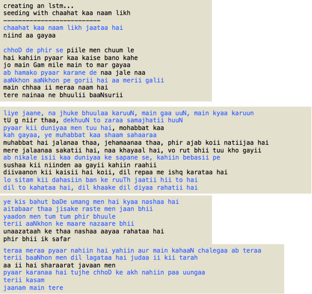
The char-rnn code generates a sequence of checkpoint files. These checkpoint files can be used to generate text, lyrics in our case, as the network proceeds with learning. Generating text file with any checkpoint file requires a short intial text string, called primetext, in char-rnn. A selected sampling of generated lyrics is shown in Figure 9. The order of these selected samplings is from early checkpoints to later checkpoints to see how well more iterations improve the resulting text. The highlighted text in blue in Figure 9 shows those segments that could be in a Bollywood lyric. Also, it is to be seen that the network is able to even generate two rhiming lines in a lyric.
Although I could have fine tuned my network by exploring with different parameter settings, I am happy with the results to conclude that RNN/LSTM can be trained, especially in certain limited domains, to produce output tending towards human-like output. Also, besides language modeling there are many other interesting applications of RNN/LSTM networks.
Finally, I would like to thank Andrej Karpathy for making his code available; otherwise this blog post wouldn’t have been written.
